Pool Testing is k-ary Search for COVID-19
I’ve seen a handful of articles in the last week about pool testing and sample pooling for COVID-19. The gist of this technique is simple: to make our limited supply of test kits (reagents) stretch farther, mix several people’s samples together and then test the mixture for COVID-19. Ideally, if the test comes back negative, everyone in that “sample pool” could be declared COVID-free using just one test. Otherwise, if the mixture comes back positive, then additional tests are needed to find the individual positive samples.
I’m far from a public health and epidemiology expert, but as an enthusiastic computer scientist I can’t help but see binary search (or more generally, $k$-ary search) all over this pool testing technique. My goal in this post is to draw out this connection, illustrating why the efficiency of $k$-ary search (and of pool testing, by extension) is so attractive. I’ll also do some crude math to explore what happens to pool testing if there are too many infections in the population and how many tests it could actually save.
If you’re not interested in any of that but want to know more about pool testing, NPR has a short primer and the FDA has put out a statement on the topic. On the other hand, if you’re interested in more serious research on the topic, this footnote1 is for you.
Finding Things Fast
In a search problem, the goal is to find a specific item $x^*$ amidst a whole bunch of possibilities $(x_1, x_2, \ldots, x_n)$. It’s like Where’s Waldo if Waldo were $x^*$ and each $x_i$ was a person on the page. Or, perhaps more practically, it’s the way you give your favorite maps app a specific address $x^*$ and it has to find that place’s data (latitude/longitude, reviews, etc.) amongst all possible places $x_i$ in its gigantic database.
A not-so-great approach to playing Where’s Waldo is to make a list of every person on the page and check them one-by-one to see if they’re Waldo. (This is, perhaps, an entertaining way to play since you get to appreciate all the fun and ridiculous details, but we’re going for efficiency here). In computer science, we call this strategy — or “algorithm” — brute force search: when all else fails, just try everything. How bad can this be? Well, in the worst case Waldo might be the very last person in our list, so we would have had to check all $n$ people before we found him. So, knowing that the least clever search strategy makes us try $n$ times before we find Waldo, can we do better?
Imagine that you have a friend who already knows where Waldo is and has agreed to help you out by telling you which half of the page he’s on (left or right). Now you only have to search half of the possibilities, or roughly $n/2$ people. Say your friend’s really helpful, and they’ll let you do this as many times as you want: they’ll keep telling you which half of the remaining section Waldo’s in until you find him. So at first you have $n$ people to look through, then after your friend helps once you have $n/2$, and after helping again you have $n/4$, and then $n/8$, and so on. In general, if your friend has helped you $i$ times, then you only have $n/(2^i)$ people to look through. Doing a little algebra, after your friend has helped you $\log_2(n)$ times, you only have $n/(2^{\log_2(n)}) = n/n = 1$ person left, and that person is Waldo. This strategy is binary search: “binary” because your friend splits the possibilities in two each time they help.
It may have been a while since you’ve brushed up on your logarithms, so let’s look at some numbers to get a sense of how fast this is. An average Where’s Waldo puzzle has roughly $n = 500$ people on it. So, if we were to use brute force search, we’d be looking through all $n = 500$ people. However, if we had our helpful friend to do binary search with us, we’d only need to ask their help $\log_2(500) \approx 9$ times before we found Waldo! Not bad, hey?
The key to binary search is in throwing away whole chunks of possibilities all at once, rapidly narrowing our search field. $k$-ary search is just a generalization, where instead of splitting the possibilities in half each time, we split them into $k$ equal parts. We then keep the $n/k$-sized section containing our target and repeat, requiring a total of $\log_k(n)$ search operations to find our target (which is even faster than binary search!). Before we call it quits with Waldo and get back to pool testing, it’s worth pointing out that there are plenty of ways to make searching even faster (especially with parallel algorithms). There are even search algorithms specifically for finding Waldo, if that’s your jam.
Pool Testing, Meet k-ary Search
Shifting our perspective on testing from personal experience (“Have I contracted COVID-19?") to the population level (“Who in our communities are positive?"), we can frame testing as a search problem. Among all individuals $(x_1, x_2, \ldots, x_n)$, we want to find those $x_i$’s that are positive for COVID-19 so they can isolate and get timely medical care. In this setting, brute force search would be individually testing every single person — and that’s way more tests than we have. The current US strategy of only testing symptomatic cases isn’t more “efficient” than brute force, it’s just brute force search on a (hopefully) small subset of the total population.
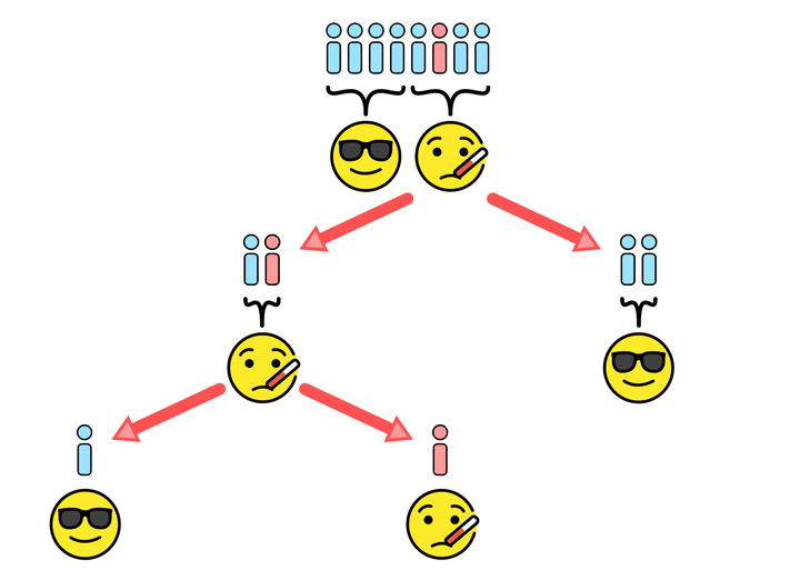
Pool testing, on the other hand, is similar to $k$-ary search. Just like our helpful friend telling us which half of the page Waldo isn’t on, a single pool test ideally shows us a whole group of people that we can declare COVID-19 negative; in our search for positive cases, we can look elsewhere.
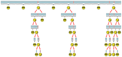
Consider the situation depicted above, with $128$ total individuals needing tests but only $4$ of them COVID-19 positive (shown in red). If we tested all $128$ people individually (brute force), we would need $128$ tests. But suppose we could reliably test pools of up to $16$ people at once, as shown in the first row. Only three of the $128/16 = 8$ pool tests would come back positive, allowing us to immediately rule out $5 \times 16 = 80$ negative individuals. For the three positive pools, we need to do additional tests to find the positive cases. This could be done by individually testing everyone in the positive pools2 — effectively using smaller brute force — requiring $3 \times 16 = 48$ additional tests. Alternatively (assuming we had enough samples), we could do pool testing again, this time on smaller pools.3 So long as there aren’t too many positive samples (something we’ll revisit shortly), this will help us save on tests: in the picture, we only end up needing $30$ additional tests to handle the $48$ individuals in positive pools. The table below compares the number of tests used by each testing strategy in this example, along with the number of samples per person required.
| Testing Strategy | Tests Used | Tests Saved | Samples per Person |
|---|---|---|---|
| Individual (brute force) | $128$ | $0\%$ | $1$ |
| Pool Testing (one round) | $56$ | $56\%$ | $1$ |
| Pool Testing (repeated) | $38$ | $70\%$ | $> 1$ |
What Can Go Wrong?
At least a few serious things:
- Added logistical complications for labs, including tracking which individuals' samples are in which pools, added mixing steps, etc.
- The possibility of larger false-negative rates (i.e., testing negative when the sample was, in fact, positive) due to samples getting diluted when they’re mixed into pools.4
- A loss of efficiency when there are too many positive samples.
For the rest of this post, I’m going to focus on that last problem. Pool testing’s strength lies in its ability to rule out large groups of negative cases at once, as we saw in the example. But with too many positive cases, the likelihood of pools testing positive becomes much higher, requiring a greater number of subsequent tests. At what point does pool testing end up using more tests than if we just tested everyone individually?
Instead of repeated pool testing (like in our example above), consider the more practical protocol of doing only one round of pool testing and then testing all samples in positive pools individually. If we have $n$ total samples, our pool size is $p$, and $x$ pool tests come back positive, then we will use a total of $n/p + xp$ tests: $n/p$ pool and $xp$ individual. Since we’d use $n$ tests doing brute force, pool testing only saves us tests if $n/p + xp < n$, or equivalently, if: $$x < (n/p)(1 - 1/p)$$
To connect the number of positive pools $x$ we’ll have based on how many positive cases are in the population, let $r$ be the probability that any given sample is COVID-19 positive. The probability that a pool of size $p$ contains a positive sample is $1 - (1 - r)^p$. There are $n/p$ total pools, so the expected (average) number of positive pools is: $$E[x] = (n/p)(1 - (1 - r)^p)$$ Therefore, we save on tests using pool testing in expectation if: $$\begin{align*} (n/p)(1 - (1 - r)^p) &< (n/p)(1 - 1/p) \\ r &< 1 - p^{-1/p} \end{align*}$$
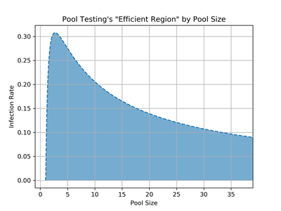
The above graph plots this efficient region. The x-axis is the pool size $p$ and the y-axis is the infection rate $r$. Any point in the blue region represents a $(p,r)$ pair for which pool testing uses less tests than brute force in expectation. For example, with a pool size of $p = 16$, our crude math suggests that pool testing is more efficient for infection rates up to, coincidentally, $r \approx 16\%$. This would be a terrifyingly high infection rate (at the time of this writing, the CDC reports a $\approx 1\%$ positive case rate in the US), so it seems that in realistic settings even one round of pool testing would save a lot of tests.
Taking Our Savings to the Bank
To recap, we’ve seen how pool testing is related to $k$-ary search, how both of these techniques leverage the ability to rule out large groups of possibilities to narrow things down quickly, and how pool testing will save us tests so long as the infection rate is low enough. The last thing to nail down is how many tests are actually saved. From our work above, we know that the expected number of tests saved using one round of pool testing is: $$\begin{align*} E[\text{# tests saved}] &= \text{# tests for brute force} - E[\text{# tests for pool testing}] \\ &= n - (n/p + E[\text{# positive pools}] \cdot p) \\ &= n - n/p - (n/p)(1 - (1-r)^p)p \\ &= n(-1/p + (1-r)^p) \end{align*}$$ The fraction of tests saved is just the number of tests saved divided by $n$, so a single round of pool testing in pools of size $p$ uses a $(1-r)^p - 1/p$ fraction less tests. The following plot shows this equation for different pool sizes $p$ as a function of the infection rate $r$.
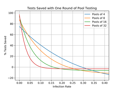
This shows that larger pool sizes have the potential for saving more tests, but also degrade in their efficiency more rapidly as the infection rate $r$ grows. Eventually, if the infection rate becomes too large, all four curves become negative and pool testing ends up using more tests than brute force. This corresponds to leaving the efficient region shown in the previous graph. If you’re having a hard time interpreting these curves, the following table compares pool testing with $p = 4$ (blue) and $p = 16$ (green).
| Pool Size | Tests Saved at $r = 1\%$ | Tests Saved at $r = 5\%$ | Infection Rate for No Savings |
|---|---|---|---|
| $p = 4$ | $71\%$ | $56\%$ | $r = 29\%$ |
| $p = 16$ | $79\%$ | $38\%$ | $r = 16\%$ |
The key takeaway is that from a purely test-savings perspective, pool testing does a remarkable job for any reasonable pool size. While it is true that pool testing can end up using more tests than traditional testing if the infection rate grows too large, my crude math suggests that the infection rate would need to be quite high ($r > 10\%$) before this inefficiency would be noticeable. At today’s US infection rate of $r \approx 1\%$, we could be $70\%$ more efficient with our limited supply of testing reagents, helping more people get tested more often. Perhaps if this technique were widely used, we would all be that much closer to safely getting on with our lives.
-
Cherif et al. 2020 detail a recent mathematical model for pool testing and Yelin et al. 2020 characterize its dilution and false-negative rates. The references in the Yelin paper also cover deeper mathematical analysis (e.g., Dorfman 1943) and how pool testing has been used to combat infectious disease in the past (e.g., for malaria in Taylor et al. 2010). ↩︎
-
From my brief sifting of the literature, practical implementations of pool testing only use one round of pool tests: roughly $65\%$ of each sample is used in a pool test, and the remaining $35\%$ is saved for an individual test in case the pool comes back positive. Repeated pool testing doesn’t seem to be used in practice, presumably because it would rely on collecting additional swab samples per person. ↩︎
-
I’ve depicted the subpool tests in a binary search kind of way where each positive pool is split in half and retested, but they could be broken into any number of groups. ↩︎
-
Yelin et al. 2020 estimate that the false-negative rates for pools as large as $16$ or $32$ is roughly $10\%$ based on their experiments. I chose not to do my speculative math for dilution and false-negative rates because I don’t understand how PCR tests actually work and don’t believe in blindly oversimplifying things for the sake of nice math. ↩︎
Joshua J. Daymude
Assistant Professor, SCAI & CBSS
I am a Christian and assistant professor in computer science studying collective emergent behavior and programmable matter through the lens of distributed computing, stochastic processes, and bio-inspired algorithms. I also love gaming and playing music.